Time to read: 9 min
Statistics may not be your favorite subject from college, but it’s a critical part of an efficient product design and manufacturing process. Using statistics you can design experiments, run tests, collect real world results, and make data-driven decisions. These experiments can be used to test the effect of changing a dimension, material, or manufacturing process step. Usually you will want to change one of these variables to improve the ability of your part to be made within tolerance or the overall performance of the product. Maybe your part keeps breaking during reliability testing, and you want to test whether changing the material reduces these failures. Or, you have to rework a large percentage of your parts, but you think that changing a dimension will make the reworks unnecessary and speed up the process. These are good opportunities to use experiments and statistics.

When we use statistics to help with our engineering designs and manufacturing processes, we go beyond mean, median, and mode to more advanced applications. One of the most useful statistics concepts is the hypothesis test, which allows you to compare results from multiple samples mathematically. This is an important part of your design process because, instead of guessing and assuming that making a change will make your product better, you can measure the effect of that change and make more informed design decisions going forward. If you’ve thoughtfully planned out your test and analysed the data properly, you’ll reach a conclusion that you can trust will improve your process, and therefore your product.
What’s a hypothesis test?
A hypothesis test is a method to test an assumption and determine whether the result is statistically significant. The assumption you’re testing can be about one population, such as assuming that the mean of the population is greater than a certain value. You can also test assumptions about two populations.
For example, you can test the assumption that the mean of one population is greater than the mean of another population. In order to test these assumptions, you gather data about a population by testing a sample of that population. Hypothesis testing can also be used to test the variance of a population, by measuring standard deviation of a sample.
Now let’s look at the steps for performing a hypothesis test. Along with these steps, we’ll also consider an engineering example. Let’s say our manufacturing partner is claiming that the mean torque of a hinge is no greater than 30 Nm. However, we have reason to believe that some of the hinge torques are greater than 30 Nm, and are therefore too strong for our application. If these hinges are being used in laptops, too strong of a torque may make it difficult to open, creating a poor user experience. So, we want to see if this is really an issue.

Step 1: Choose your test
The type of test you use (and the corresponding test statistic) will depend on what you are trying to learn and the sample you can collect. For our example, let’s say we’re able to test 20 hinges, so we’ll start with a t-test with a sample size of 20.
T-test
The t-test, or student’s t-test, is useful when you have a smaller sample size. Sample sizes larger than 30 allow you to assume a normal distribution, but sometimes it is impossible to collect more than 30 data points. A t-test assumes a t-distribution, which works with a smaller sample size. In this case, you estimate the population variance from your sample standard deviation. A t-test can be used to compare the mean of the sample to a given or known value. You can also do a two sample t-test to compare the means of two groups.
Z test
A Z test is used to test the mean of a population, or compare the means of two populations. For this test, the population should be normally distributed (or you’ll need a sample size over 30). With sample sizes over 30, you can assume that the sample is normally distributed and that the sample standard deviation is equal to the population variance.
F test
The F-test is used to compare the standard deviations of two samples. This can be useful when you want to compare the variability of two designs to see which one has less variation. An F-test can also be used for sample sizes smaller than 30.
Chi-square
So far, all of the tests discussed require quantitative data, or continuous numerical results. The chi-square test, on the other hand, compares categorical data. Examples of categorical data include age group, education level, or marital status. Chi-square tests require larger sample sizes. The actual number depends on the amount of categories, but a good starting point is 50 or more data points.
Step 2: State your hypotheses
Once you’ve chosen your test, you’ll want to state your hypotheses (a good necessary first step in any experiment). You’ll always have two hypotheses: a null hypothesis and an alternative hypothesis. The null hypothesis is usually what you want to disprove, and often states that there is no change or difference. The alternative hypothesis is what you think might be true based on a change you made or some other changed factor. Another way to frame it: the null hypothesis states that there’s no effect, and the alternative hypothesis states that there is an effect.
Here are the hypotheses for our hinge example:
Null hypothesis (H0): μ < μ0 , where μ0 = 30 Nm
Alternative hypothesis (H1): μ > μ0
Step 3: Choose a significance level (α)
This is the level at which you will determine the results are statistically significant. In the next step, you’ll calculate the p-value, which you compare to α. α = 0.05 is a very commonly used significance level because it will usually give you a small enough probability of getting a Type I error (discussed below) while also capturing small, but still significant, differences between the mean of the sample and the null hypothesis. Advanced statistics concepts can be used to determine the best significance level for the application, but for this example we will stick with the conventional value.
Step 4: Calculate the test statistic
This test statistic depends on the hypothesis test you chose. For the t-test, the test statistic is the variable t, calculated using the formula below. In this formula, x-bar is the mean of the sample, μ0 is our null hypothesis, S is the standard deviation of the sample, and n is the sample size.
You’ll then use this test statistic, t, to calculate the p-value, or the probability of getting that specific test statistic value by random chance if the null hypothesis is true. Next, compare this p-value to the significance level.
Let’s say we randomly selected 20 hinges to measure. Here are the measurements:
| 26.42 | 31.16 | 30.57 | 30.82 | 30.51 |
| 31.46 | 30.46 | 30.94 | 32.34 | 30.75 |
| 29.72 | 28.18 | 33.1 | 31.21 | 28.8 |
| 29.71 | 30.8 | 31.35 | 31.64 | 29.42 |
For our example, we will use data we collected and the formula for the t-test:

X-bar represents the mean of the sample (30.7 BM = Nm). μ0 is the null hypothesis, which in this case is 30 Nm. S is the standard deviation of the sample (in this case 1.1), and n = 20 is the sample size. After filling in these values we get t = 2.6. To find the p-value from our t statistic, you can use a table to look up the p-value, or a formula in Excel to calculate it. In our example, we get a p-value of 0.0052, which is less than our α = 0.05 significance level. So, we can reject the null hypothesis and conclude that we are 99.48% confident that the mean torque of the hinges is greater than 30.
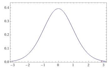
The graph below shows where the t statistic that we calculated falls on a distribution. The shaded part is the probability of getting this result by random chance. Again, this probability is below our significance level of 0.05.

Step 5: Interpret the results
When running a hypothesis test, you have two options for results: you can reject your null hypothesis or fail to reject the null hypothesis. Notice that rejecting the null hypothesis doesn’t mean you’re able to accept the alternative hypothesis; instead, you are disproving the null hypothesis. This may seem convoluted, but statistics requires very specific language in order to be clear about the results. The data you collect merely proves the null hypothesis wrong rather than proving the alternative hypothesis correct.
In order to reject the null hypothesis, the p-value needs to be smaller than alpha, the significance level. A smaller p-value tells us that the probability of the null hypothesis occurring by random chance is too small to be reasonable. Therefore, if p < α, you reject the null hypothesis. However, if the p-value is greater than or equal to α, you fail to reject the null hypothesis. In other words, there is not enough evidence to conclude that there is a difference between the null hypothesis and the measured mean of the sample.
Even with meticulously planned experiments, it’s possible to make mistakes. With hypothesis tests, the data comes from a sample rather than an entire population, and it’s possible for the sample to misrepresent the population. There are two types of errors that can be made with hypothesis testing: Type I and Type II errors.
| Null hypothesis is true | Null hypothesis is false | |
| p < α | Type I Error: False positive | Correct decision, effect exists |
| p > α | Correct decision, no effect | Type II Error: False negative |
We can use the example of a smoke detector to represent the hypothesis test in these four situations. When the smoke detector is working, it goes off when there is smoke and it doesn’t go off when there is no smoke. However, if the smoke detector goes off, but there is no smoke, you have a Type I error, or a false positive. In other words, the test is detecting an effect or a difference when there is nothing there.
In our example of the hinge, a Type I error would occur if, although we came to the conclusion that the average hinge torque is greater than 30 Nm, the average hinge torque was actually less than or equal to 30 Nm. So, we would have detected a significant difference even if there wasn’t one. This would cause us to believe we need to make some kind of change in the hinge to reduce the torque, which might result in hinges that are now too weak to support the opening and closing of a laptop.
On the other hand, if there is smoke and the smoke detector does not go off, it’s a false negative, or a Type II error. In the case of a hypothesis test, the test is not detecting a significant difference when there is one.
Again, in our hinge example, a Type II error would occur if we wrongly concluded that our hinges were less than or equal to 30 Nm, on average. This would mean that we would use hinges that are too strong, resulting in laptops that are difficult to open.
These errors are hard to detect when they happen, but there are ways to design the hypothesis test to make these errors less likely. The probability of getting a false positive is the same as the significance level, α. Therefore, by decreasing the significance level, you can decrease the likelihood of encountering a Type I error.
The probability of a Type II error is more difficult to estimate because small sample sizes or high data variability can cause false negatives. Type II errors are more difficult to reduce, which is why it’s critical to create a well-designed test and minimize your chance of error.
Conclusion
Hypothesis testing is so powerful because it uses statistics and data that you gather to help you make informed, data-driven decisions about whether your design and manufacturing process is producing parts as you expect. Performing these hypothesis tests can help you find issues and determine whether your changes are leading to improvements. In the example of our hinges, we were able to determine that the torque was significantly higher than what we wanted. In the real engineering world, this would lead to further steps of making design changes to improve those hinges, resulting in a better product. If you follow these steps, you’re on your way to an experiment and analysis that will help improve your designs and streamline your manufacturing process.
For more useful engineering articles, sign up for Fictiv’s monthly newsletter below!


